Custom Visualization
For each window being processed, Lancet2 can optionally serialize two types of graphs that are generated during the variant calling process. This can be enabled by passing a .tar.gz archive path to the --out-graphs-tgz flag — Lancet writes a single gzipped TAR bundle containing the per-window outputs:
-
the kmer-based colored de-bruijn overlap graph after the cleaning/pruning steps of the assembly process serialized as
DOTformatted graphviz files. One DOT file per connected component per window — eitherenumerated_walks(when haplotype walks were successfully enumerated) orfully_pruned(when assembly stopped before walks could be enumerated). -
the sequence graph generated from the multiple sequence alignment of all the assembled contigs from the de-bruijn graph assembly serialized as
GFAformatted files.
Lancet2 pipeline --reference ref.fasta \
    --tumor tumor.bam --normal normal.bam \
    --region "chr22" --out-graphs-tgz output-graphs.tar.gz
Why TAR.GZ instead of a directory tree
On shared filesystems (e.g. GPFS), per-file mkdir + openat operations serialize at the metadata server and add many minutes of unavoidable overhead at typical --num-threads settings when graph outputs are written as per-window files in a directory tree. Bundling all outputs into a single gzipped TAR archive cuts the metadata cost from ~hundreds-of-thousands of operations to two per worker (one open + one close), shifts the bottleneck from metadata-bound to sequential-write-bandwidth-bound, and as a side benefit gets a ~2-4× storage win from gzip compression of the text-heavy DOT/GFA/FASTA streams.
Extracting the archive
Once Lancet2 finishes, extract the archive to recover the original per-window directory tree:
(Modern GNU tar auto-detects gzip via the .gz suffix, so -xf works in place of -xzf on most systems.)
The extracted tree has two top-level subdirectories:
-
dbg_graph/${CHROM}_${START}_${END}/—DOTfiles for each component:dbg__${CHROM}_${START}_${END}__${STAGE}__k${KMER_SIZE}__comp${COMP_ID}.dot, where${STAGE}isenumerated_walks(walks enumerated successfully) orfully_pruned(graph pruned but no walks). Snapshots are written only for the k-attempt that succeeded — abandoned attempts (cycle / complexity retry) leave no artifacts in the archive. -
poa_graph/${CHROM}_${START}_${END}/—GFAfiles for each component:msa__${CHROM}_${START}_${END}__c${COMP_ID}.gfa. Each component subdirectory also contains aFASTAfile with the raw multiple sequence alignment output.
For ad-hoc inspection of a single file without full extraction:
tar -xzOf output-graphs.tar.gz dbg_graph/chr22_X_Y/dbg__chr22_X_Y__enumerated_walks__k31__comp0.dot \
  | dot -Tpdf -o my_window.pdf
DOT snapshot verbosity
The --graph-snapshots flag controls how much of the graph pruning pipeline gets serialized. Two values are accepted:
final(default) — emits exactly one DOT file per component per window:enumerated_walksorfully_pruned.verbose— additionally emits intermediate-stage snapshots after each post- compression pruning boundary (compression1,low_cov_removal2,compression2,short_tip_removal). Pre-compression stages are not snapshot — those graphs have tens of thousands of nodes per window and are unusable as rendered DOT.
# Default: one DOT per component per window
Lancet2 pipeline ... --out-graphs-tgz output-graphs.tar.gz

# Verbose: adds the four post-compression stages too
Lancet2 pipeline ... --out-graphs-tgz output-graphs.tar.gz --graph-snapshots verbose
Inspecting DOT formatted assembly graphs
The DOT files can be rendered in the pdf format using the dot utility available in the graphviz visualization software package. The DOT file can also be exported to various other output formats with the dot utility tool.
The above command will create a example_file.pdf file that shows the de-bruijn assembly graph.
Visual encoding
Lancet2's DOT output uses orthogonal styling axes so multiple signals can stack on a single node without losing information:
| Concern | Source | Visual encoding |
|---|---|---|
| Sample role | Node::IsCaseOnly / IsCtrlOnly / IsShared / HasTag(REFERENCE) | fillcolor (indianred / mediumseagreen / steelblue / lightblue) |
| Source/sink anchor | mSourceAndSinkIds | heavy goldenrod border + double peripheries |
Probe-marked k-mer (--probe-variants) | ProbeTracker::GetHighlightNodeIds | style="filled,striped" with orchid stripe accent |
| Walk membership (per edge) | enumerated haplotype walks | graphviz native colorList (color="#A:#B:#C") — parallel-color stripes |
A probe-marked anchor in a CASE-only k-mer renders all three signals simultaneously: indianred fill + heavy goldenrod border + striped orchid accent. No signal is lost to overlay precedence.
Walk overlay (enumerated_walks files)
Each enumerated haplotype walk is colored with a maximally-distinct hex color chosen from a 64-entry palette pre-computed via k-means clustering in CIE L*a*b* perceptual color space (see scripts/gen_walk_palette.py). The reference walk (index 0) gets a fixed white accent (#FFFFFF) so it stands out as the backbone; ALT walks consume the LAB palette starting at index 1.
When multiple walks share an edge, graphviz's native colorList renders the edge as parallel-color stripes — the edge picks up all the walks that traverse it, not just the dominant one. The bidirected mirror of every walked edge is colored with the same style, so under the neato layout both anti-parallel splines carry the walk's color.
Verbose-mode intermediate stages
When --graph-snapshots=verbose is set, four additional DOT files per component trace the graph through the pruning pipeline:
| Stage filename label | Captured after |
|---|---|
compression1 | First unitig compression |
low_cov_removal2 | Second pass low-coverage node removal |
compression2 | Second unitig compression |
short_tip_removal | Tip removal (recursive until stable) |
Pre-compression stages (initial build, first low-coverage removal, anchor discovery) are intentionally not snapshot — they have too many nodes to render usefully. The first usable snapshot is compression1, after the graph collapses into unitigs.
# Render every snapshot to PDF
for dot_file in output-graphs/dbg_graph/*/*.dot; do
    dot -Tpdf -o "${dot_file%.dot}.pdf" "${dot_file}"
done
Inspecting GFA formatted sequence graphs
The generated GFA files can be visualized in Bandage or BandageNG.
The GFA file generated by Lancet2 is chopped i.e the nodes are in their decomposed form. They need to be unchopped using the vg toolkit, before they can be visualized or used in other downstream processes. Below is a command to unchop the Lancet2 GFA graph.
BandageNG
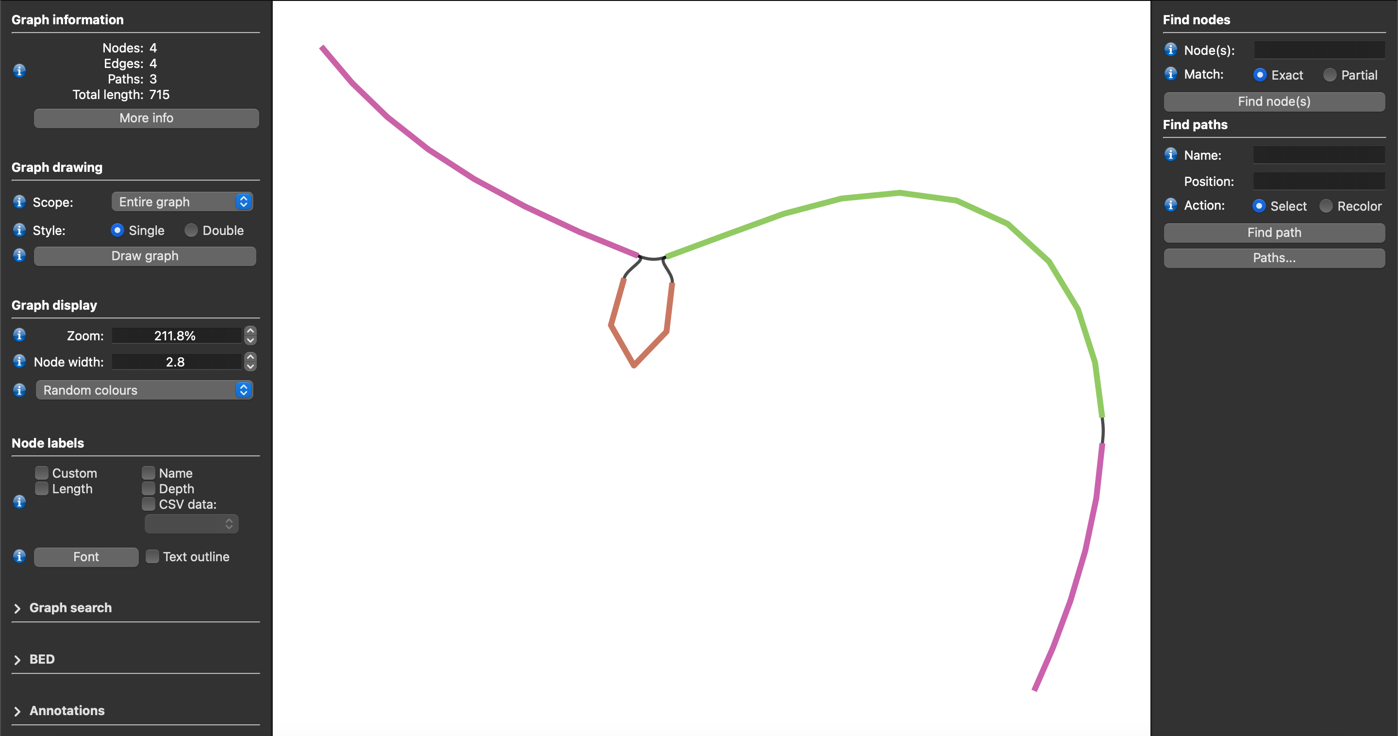
The image above shows a screenshot of an unchopped Lancet2 sequence graph in GFA format visualized using the BandageNG toolkit.
Sequence Tube Map
Lancet2 addresses the longstanding challenge of visualizing variants along with supporting reads from multiple samples in graph space. Users can easily load the unchopped GFA formatted graphs into the Sequence Tube Map environment allowing somatic variants' visualization along with their supporting read alignments from multiple samples.
The following steps describe the workflow to visualize Lancet2 variants of interest in graph space using the Sequence Tube Map framework.
-
Install prerequisite tools – Lancet2 (https://github.com/nygenome/Lancet2), samtools, bcftools, vg version 1.59.0, and jq, and ensure that they are available as commands that can be executed in the environment PATH.
-
Install Sequence Tube Map (https://github.com/vgteam/sequenceTubeMap) version 0452ecb82d057372e359a9b456d789336e5ab8a1.
-
Use the Lancet2's
prep_stm_viz.shscript to run Lancet2 on a small set of variants of interest that need to be visualized in Sequence Tube Map. The script will run Lancet2 using the--out-graphs-tgzflag, thentar -xzfthe resulting archive to recover the GFA-formatted sequence graphs for each variant of interest. Local VG graphs and indices required to load the sample reads along with the Lancet2 graph are then constructed enabling simplified use with "custom" data option in Sequence Tube Map interface. -
After running the Sequence Tube Map Server as detailed in the Tube Map Readme, set “Data” to “custom” and “BED file” to “index.bed”. Pick a “Region”(or variant) of interest and hit “Go” to visualize.
Demo Sequence Tube Map server
Sequence Tube Map demo server containing somatic variants from COLO829 tumor/normal pair sample can be found at this link – https://shorturl.at/JQZsy