Custom Visualization
For each window being processed, Lancet2 can optionally serialize two types of graphs that are generated during the variant calling process. This can be enabled by passing a non-existing directory to the --graphs-dir flag to write per window serialized graphs in the directory.
-
the kmer-based colored de-bruijn overlap graph after the cleaning/pruning steps of the assembly process serialized as
DOTformatted graphviz files. OneDOTfile is generated for every strongly connected component for each window. -
the sequence graph generated from the multiple sequence alignment of all the assembled contigs from the de-bruijn graph assembly serialized as
GFAformatted files.
Lancet2 pipeline --reference ref.fasta \
    --tumor tumor.bam --normal normal.bam \
    --region "chr22" --graphs-dir output-graphs
The above command will create two directories named dbg_graph and poa_graph in the provided output-graphs directory.
-
In the
dbg_graphdirectory, you will find theDOTfiles generated for each window –dbg__${CHROM}_${START}_${END}__fully_pruned__k${KMER_SIZE}__comp${COMP_ID}.dot -
In the
poa_graphdirectory, you will find theGFAfiles generated for each window –msa__${CHROM}_${START}_${END}__c${COMP_ID}.gfaThepoa_graphalso contains aFASTAfile with the raw multiple sequence alignment output.
Info
If you are interested to further debug the de-bruijn graph assembly process, you can generate DOT files for the all the intermediate steps before the fully_pruned graph is generated, by re-compiling the Lancet2 binary in Debug mode using -DCMAKE_BUILD_TYPE=Debug instead of -DCMAKE_BUILD_TYPE=Release in the cmake step.
The intermediate states that can be inspected in their order of generation are as follows – low_cov_removal1, found_ref_anchors, compression1, low_cov_removal2, compression2, short_tip_removal.
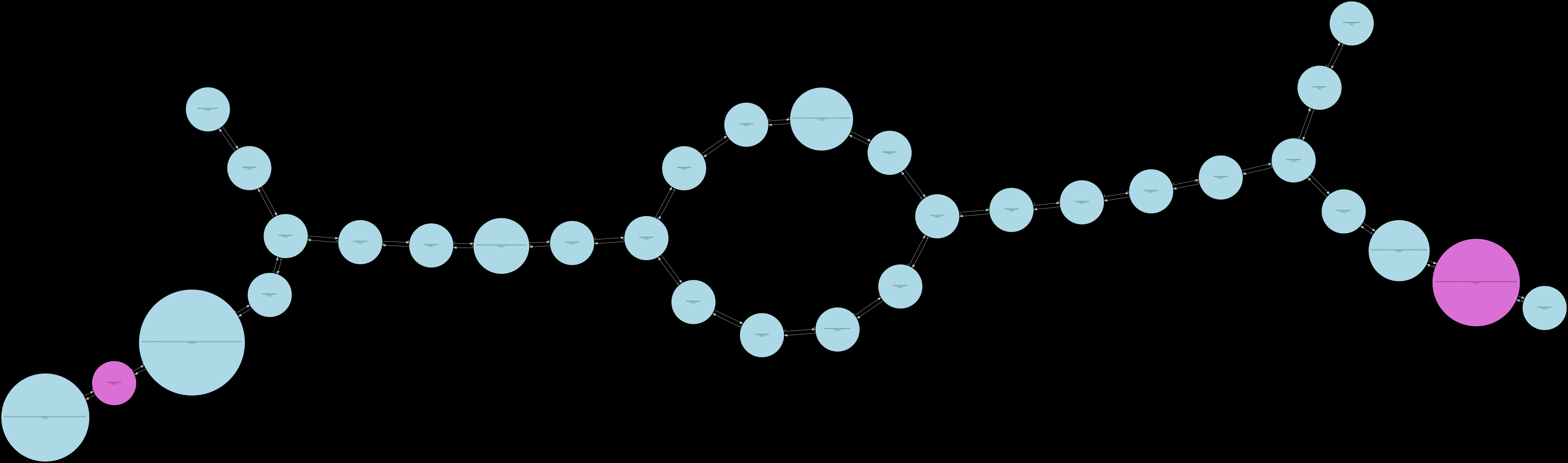
Inspecting DOT formatted assembly graphs
The DOT files can be rendered in the pdf format using the dot utility available in the graphviz visualization software package. The DOT file can also be exported to various other output formats with the dot utility tool.
dot -Tpdf -o example_file.pdf example_file.dot
The above command will create a example_file.pdf file that shows the de-bruijn assembly graph.
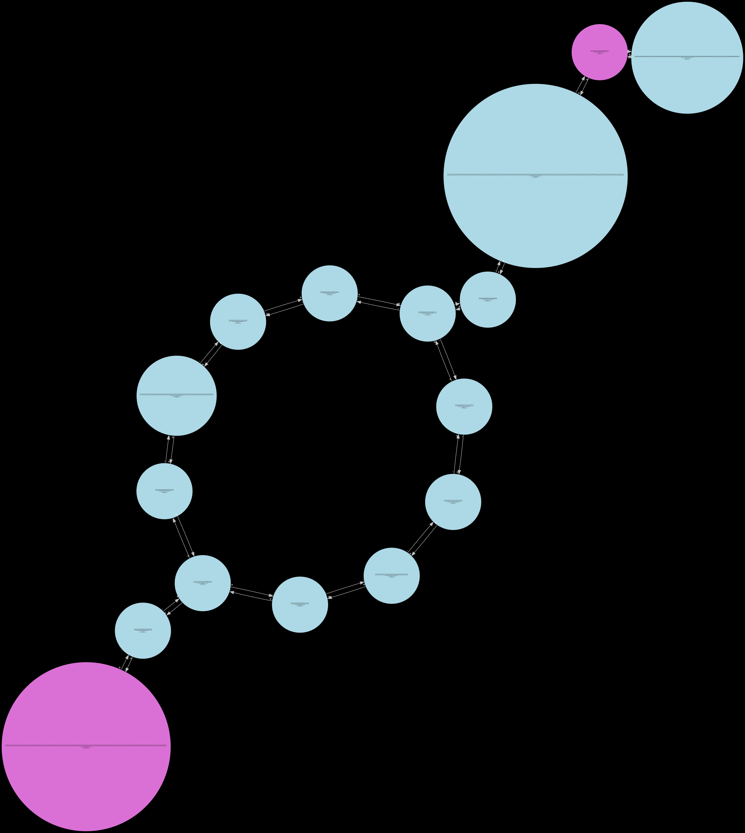
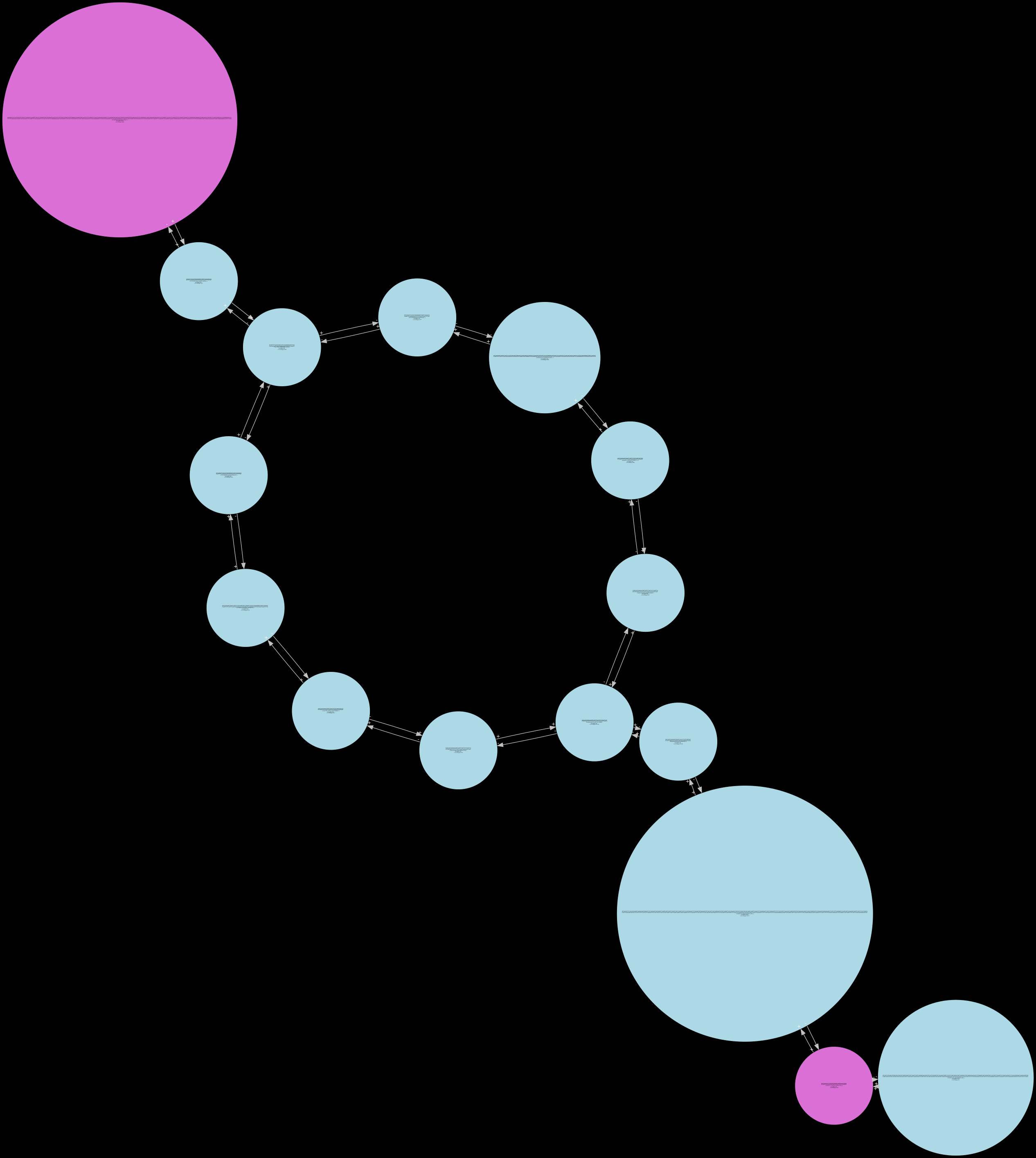
Shown below are the renderings of the de-bruijn assembly graph through all of it's intermediate states (can only be visualized in Debug mode Lancet2 binary. ideal for small regions.).
Note
Only the fully_pruned graph will be serialized when the standard Release build is used. The remaining 6 other states can only be visualized in the Debug build of Lancet2. The Debug build is much slower than the standard Release build and is only recommended to be used on small regions for inspection.
low_cov_removal1
found_ref_anchors
compression1
low_cov_removal2
compression2
short_tip_removal
fully_pruned
Inspecting GFA formatted sequence graphs
The generated GFA files can be visualized in Bandage or BandageNG.
The GFA file generated by Lancet2 is chopped i.e the nodes are in their decomposed form. They need to be unchopped using the vg toolkit, before they can be visualized or used in other downstream processes. Below is a command to unchop the Lancet2 GFA graph.
vg mod --unchop ${INPUT_GFA} > ${OUTPUT_GFA}
BandageNG
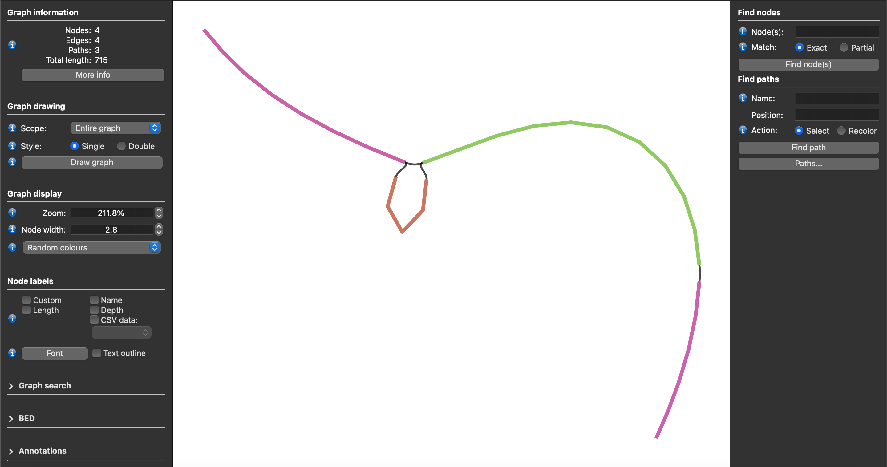
The image above shows a screenshot of an unchopped Lancet2 sequence graph in GFA format visualized using the BandageNG toolkit.
Sequence Tube Map
Lancet2 addresses the longstanding challenge of visualizing variants along with supporting reads from multiple samples in graph space. Users can easily load the unchopped GFA formatted graphs into the Sequence Tube Map environment allowing somatic variants' visualization along with their supporting read alignments from multiple samples.
The following steps describe the workflow to visualize Lancet2 variants of interest in graph space using the Sequence Tube Map framework.
-
Install prerequisite tools – Lancet2 (https://github.com/nygenome/Lancet2), samtools, bcftools, vg version 1.59.0, and jq, and ensure that they are available as commands that can be executed in the environment PATH.
-
Install Sequence Tube Map (https://github.com/vgteam/sequenceTubeMap) version 0452ecb82d057372e359a9b456d789336e5ab8a1.
-
Use the Lancet2’s prep_stm_viz.sh script to run Lancet2 on a small set of variants of interest that need to be visualized in Sequence Tube Map. The script will run Lancet2 using the --graph-dir flag to generate GFA formatted sequence graphs for each variant of interest. Local VG graphs and indices required to load the sample reads along with the Lancet2 graph are then constructed enabling simplified use with “custom” data option in Sequence Tube Map interface.
-
After running the Sequence Tube Map Server as detailed in the Tube Map Readme, set “Data” to “custom” and “BED file” to “index.bed”. Pick a “Region”(or variant) of interest and hit “Go” to visualize.
Demo Sequence Tube Map server
Sequence Tube Map demo server containing somatic variants from COLO829 tumor/normal pair sample can be found at this link – https://shorturl.at/JQZsy